Shape comparison
The key operations performed by ampscan are used for comparison betweem two shapes. To do this, we need to first align the shapes.
[1]:
from ampscan import AmpObject, align, registration
[2]:
import warnings
warnings.filterwarnings('ignore')
%matplotlib inline
[3]:
base = AmpObject('stl_file.stl')
move = AmpObject('stl_file_2.stl')
# These are already pre-aligned so add some rotation
move.rotateAng([20, -30, 10], ang='deg')
Alignment
Then we create the alignment object, although we don’t want to run the ICP algorithm yet so we set maxiter=0. By default, when you create the align object it will run the algorithm with the passed variables
[4]:
al = align(move, base, maxiter=0)
[5]:
import matplotlib.pyplot as plt
plt.axis('off')
im = al.genIm(crop='False')[0]
ax = plt.imshow(im, interpolation='bicubic')
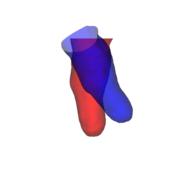
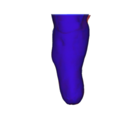
As we can see, the two scans are misaliged. We can then call the ICP method on the align object and re-render
[6]:
al.runICP()
al.s.addActor()
al.m.addActor()
plt.axis('off')
im = al.genIm(crop='False')[0]
ax = plt.imshow(im, interpolation='bicubic')
Registration
Following alignment, we can then perform a registration stage which then enables direct shape comparison between the two shapes. First, we create the registration object, this automatically runs the registration step.
[7]:
reg = registration(al.s, al.m, steps=10, neigh=10, smooth=1)
reg.reg is the AmpObject resulting from the registration, with the displacement field stored in the values attribute. This can then be plotted with a scalar bar
[8]:
plt.axis('off')
reg.reg.createCMap()
reg.reg.addActor(CMap=reg.reg.CMapN2P)
reg.reg.actor.setScalarRange([-4, 4])
im, win = reg.reg.genIm(out='im')
win.setScalarBar(reg.reg.actor)
win.Render()
im = win.getImage()
ax = plt.imshow(im, interpolation='bicubic')
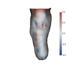
Now we’ve compared the two shapes we can now analyse the shape in more detail