Analysis

ampscan offeres several methods for analysis of the shapes. This analysis can then be plotted using matplotlib

from ampscan import AmpObject, align, registration, analyse
import numpy as np

import warnings
warnings.filterwarnings('ignore')
%matplotlib inline

base = AmpObject('stl_file.stl')
targ = AmpObject('stl_file_2.stl')

Slicing

The analysis code is mostly dependent upon the way in which the scan is sliced into 2D shapes. The examples below show the effect of using coarse or fine slicing

import matplotlib.pyplot as plt
coarse = analyse.create_slices(base, [0.1, 0.9], 0.1, typ='norm_intervals')
fine = analyse.create_slices(base, [0.01, 0.99], 0.01, typ='norm_intervals')

fig = plt.figure()
ax1 = fig.add_subplot(1, 2, 1, projection='3d')
for p in coarse:
    ax1.plot(p[:,0],
             p[:,1],
             p[:,2],
             color=[31.0/255, 73.0/255, 125.0/255])
ax1.set_title('Coarse')
ax2 = fig.add_subplot(1, 2, 2, projection='3d')
ax2.set_title('Fine')
for p in fine:
    ax2.plot(p[:,0],
             p[:,1],
             p[:,2],
             color=[170.0/255, 75.0/255, 65.0/255])

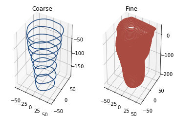
As you can see, the number of slices used make a clear visual difference to the shape. We can then calculate several metrics.

Volume, Cross-section area and Widths

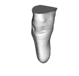
The volume can be estimated from the slices or computed directly if the surface is closed. If the surface is not closed, a simple hole filling algorithm is run. The closed shape can be returned by the function as shown below.

true_vol, closed = analyse.calc_volume_closed(base, return_closed=True)
plt.axis('off')
im = closed.genIm(out='im', az=20, el=20)[0]
ax = plt.imshow(im, interpolation='bicubic')

We can estimate the volume based upon the slices we have generated or directly with the hole filling algorithm

fig, ax = plt.subplots()
ax.bar((0, 1, 2), (analyse.est_volume(coarse), analyse.est_volume(fine), true_vol), color=[31.0/255, 73.0/255, 125.0/255])
ax.set_xticks([0, 1, 2])
ax.set_xticklabels(['Coarse', 'Fine', 'True'])
ax.set_ylabel('Volume mm³')
None

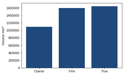
As you can see the number of slices used makes a large difference to the volume in this case!

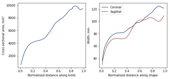
Then we can plot the cross-sectional area and both the coronal and sagittal widths

fig, (ax1, ax2) = plt.subplots(1, 2)
fig.set_size_inches(9, 4)
ax1.plot(np.arange(0.01, 0.99, 0.01), analyse.calc_csa(fine), color=[31.0/255, 73.0/255, 125.0/255])
ax1.set_xlabel('Normalised distance along kimb')
ax1.set_ylabel('Cross sectional area, mm²')
cor, sag = analyse.calc_widths(fine)
ax2.plot(np.arange(0.01, 0.99, 0.01), cor, color=[31.0/255, 73.0/255, 125.0/255], label='Coronal')
ax2.plot(np.arange(0.01, 0.99, 0.01), sag, color=[170.0/255, 75.0/255, 65.0/255], label='Sagittal')
ax2.set_xlabel('Normalised distance along shape')
ax2.set_ylabel('Width, mm')
ax2.legend()
None

Registration analysis

Finally we can also analyse the distribution of shape deviation between shapes, with colour corresponding to the 3D visualisation

reg = registration(base, targ, steps=10, neigh=10, smooth=1)

c1 = [31.0, 73.0, 125.0]
c3 = [170.0, 75.0, 65.0]
c2 = [212.0, 221.0, 225.0]
CMap1 = np.c_[[np.linspace(st, en, 6) for (st, en) in zip(c1, c2)]]
CMap2 = np.c_[[np.linspace(st, en, 6) for (st, en) in zip(c2, c3)]]
CMap = np.c_[CMap1[:, :-1], CMap2]/255

fig, ax = plt.subplots()
N, bins, patches = ax.hist(reg.reg.values, bins=11, range=(-5.5, 5.5), density=True)
ax.set_xlabel('Shape deviation, mm')
ax.set_ylabel('Probability density')

for i, p in enumerate(patches):
    p.set_facecolor(CMap[:, i])

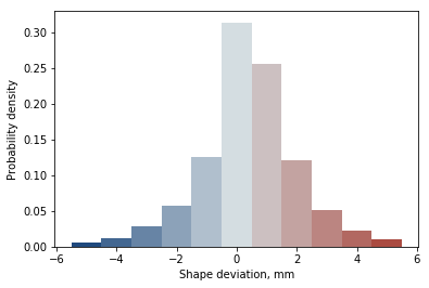
There we have it, this is the basic functionality of ampscan. Much of this can be accessed using the webapp, or there’s way more you can do with your own analysis. Enjoy!